

In geochemistry, clusters of anomalous samples are often taken as validation. If multiple nearby samples return elevated values, the interpretation feels straightforward: we are likely over the top of a mineralized system. This intuition is not wrong. Hydrothermal systems are inherently spatial, and processes such as alteration, fluid flow, and metal dispersion generate continuous geochemical footprints. In that sense, spatial autocorrelation (where nearby samples are more similar than distant ones) is exactly what we expect to see over mineralization.
The issue is that spatial autocorrelation is not unique to mineralization. It is a fundamental property of nearly all spatial datasets. Lithology, topography, weathering profiles, and even sampling design introduce spatial structure into geochemical data. As a result, clusters of anomalous values can emerge even in completely unmineralized systems. This means that the presence of a cluster, on its own, does not confirm geological significance. In fact, because geochemical datasets are almost always spatially dependent, treating samples as independent can lead to overconfidence in patterns that are simply artifacts of proximity rather than indicators of mineralization. This is a well-recognized issue in spatial modelling, where ignoring spatial autocorrelation can produce results that appear robust but fail when applied beyond the sampled locations.
The key shift, then, is not to reject clustering, but to contextualize it. Instead of asking whether anomalies are clustered, the more meaningful question is whether the observed clustering is stronger, more coherent, or more structured than what would be expected from spatial autocorrelation alone. This reframes spatial autocorrelation from being evidence of mineralization into being a baseline against which anomalies must be evaluated.
A practical workflow begins with explicitly characterizing that baseline. The first step is to quantify global spatial autocorrelation using a metric such as Moran’s I. This provides a dataset-level understanding of whether values are spatially clustered, random, or dispersed. In many geochemical datasets, Moran’s I will already indicate strong positive autocorrelation, meaning that clustering is expected. Recognizing this upfront prevents the misinterpretation of clusters as inherently meaningful.
The next step is to move from global to local analysis. Local indicators of spatial association, such as Local Moran’s I, allow the dataset to be decomposed into spatial relationships at the sample scale. This enables the identification of high–high clusters, where elevated values are surrounded by similarly elevated values, as well as spatial outliers, where high values occur in otherwise low backgrounds. This distinction is critical. Broad high–high regions may reflect lithological or regolith controls, whereas isolated or structurally aligned clusters may be more indicative of focused mineralizing processes.
To further constrain whether anomalies are meaningful, the spatial continuity of the data must be quantified. This is where variography becomes essential. By examining how similarity between samples decays with distance, the variogram defines the natural spatial correlation range of the system. This range represents the distance over which samples are expected to be similar due to background processes. From an exploration perspective, this provides a powerful filter: anomalies that extend beyond the natural correlation range, or that show internal gradients within that range, are more likely to reflect mineralized systems rather than background variability.
Once spatial structure is defined, anomaly detection can be reframed in a spatial context. Instead of applying thresholds globally, anomalies can be evaluated relative to their spatial neighborhood. This can be done by comparing sample values to local background statistics, identifying residuals from spatial trends, or integrating clustering results with geological constraints. At this stage, geochemistry should not be interpreted in isolation. Structural data, lithology, and alteration patterns should be brought in to assess whether identified clusters align with plausible geological controls, such as fault zones, permeability pathways, or reactive host rocks.
The final step is integration and decision-making. A target gains confidence not simply because it is anomalous or clustered, but because it satisfies multiple spatial criteria: it exceeds background spatial autocorrelation, persists across meaningful distances, exhibits internal coherence or gradients, and aligns with a geological framework that supports fluid flow and metal deposition. Conversely, clusters that mirror sampling density, follow topographic gradients, or remain confined within the expected spatial correlation range should be treated with caution.
This workflow represents a shift in how geochemical anomalies are evaluated. Instead of using spatial clustering as confirmation, spatial autocorrelation is treated as a starting point; something to be measured, understood, and accounted for. The question is no longer whether anomalies cluster, but whether they behave in a way that cannot be explained by spatial structure alone. That distinction is subtle, but it is ultimately what separates noise from signal and targets worth drilling from those that are simply well sampled.
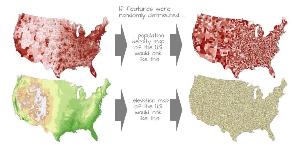
Image credit: Manuel Gimond https://mgimond.github.io/Spatial/index.html